Differentiate Categorical Variables From Continuous Variables in Sas
Categorical
We generally think of data as a collection of "measurements," in a loose sense of the word "measurement". In this loose sense, there are two basic types of "measurement", measurements on continuous scales, and measurements on categorical scales. (In ordinary speech the word "measurement" often implies a continuous scale.)
Continuous measurements can be represented by a point on a number line, are well-ordered, and in principle can take on one value of an infinite set of choices. Think of a variable like age, which varies continuously from 0 to higher numbers, and where there is a unique order to the ages represented by 1, 5.5, and 55. In principle we can measure age with arbitrary precision - 5.5, or 5.5001 or 5.5000001. The scale here might be measured in days or years, but in any case it is continuous.
Categorical measurements can be represented by arbitrary labels (maybe numerals, maybe character strings), have no conceptual order, and take one value from a finite set of choices. Think of a variable like state of residence, which takes one of about 50 values (Washington, D.C.? Territories?), which have no inherent order.
(Interval and ordinal measurements may be thought of, and are often treated, as continuous measurements with limited precision.)
The distinction between continuous and categorical variables is fundamental to how we use them the analysis. In a regression for example, continuous variables give us slopes and curvature terms, where categorical variables give us intercepts.
In R, it is convenient to manage categorical data as factors. In software like Stata, SAS, and SPSS, we specify which variables are categorical when we call an analytical procedure like regression - no special distinction is made when we are managing or storing our data. In R, we specify which variables are factors when we create and store them - in an analytical procedure we need make no additional specification to distinguish levels of measurement.
In R, a factor refers to a class of data stored in numeric form, usually with some sort of value labels. The numbers (integers) merely represent distinct categories, with no meaningful order to the categories.
For example, we might have a data set where '1' means Green Bay, '2' means Madison, and '3' means Milwaukee.
As with Date class data, we will seldom need to manipulate the underlying integers, we will mainly work with the "human-readable" value labels.
The basic constructor function for data with class factor is factor(). For example, we can begin with a character vector of city names, and use factor() to construct a factor from this.
city <- c("Madison", "Milwaukee", "Green Bay") city [1] "Madison" "Milwaukee" "Green Bay" x <- factor(city) x [1] Madison Milwaukee Green Bay Levels: Green Bay Madison Milwaukee Notice that factors print differently than character data - no quotes.
Factors in Generic Functions
In addition to printing slightly differently than character data, in generic functions that take numeric inputs, factors are treated differently as well. Three functions that give different output with factors (versus a numeric vector) are summary(), plot(), and lm().
We can look at the example data set chickwts, which includes both a numeric variable and a factor variable. We learn from help(chickwts) that this data set was created from an experiment testing the effect of different feeds on chicken weights.
Using the summary function, the factor feed produces a frequency table, rather than the six number summary produced by weight.
str(chickwts) # "weight" is numeric, "feed" is categorical 'data.frame': 71 obs. of 2 variables: $ weight: num 179 160 136 227 217 168 108 124 143 140 ... $ feed : Factor w/ 6 levels "casein","horsebean",..: 2 2 2 2 2 2 2 2 2 2 ... head(chickwts) weight feed 1 179 horsebean 2 160 horsebean 3 136 horsebean 4 227 horsebean 5 217 horsebean 6 168 horsebean summary(chickwts) weight feed Min. :108.0 casein :12 1st Qu.:204.5 horsebean:10 Median :258.0 linseed :12 Mean :261.3 meatmeal :11 3rd Qu.:323.5 soybean :14 Max. :423.0 sunflower:12 In plots, a factor produces a categorical x-axis, and a boxplot rather than a scatter plot.
plot(weight ~ feed, data = chickwts) 
In modeling, a factor is used as a categorical variables, generating a set of dummy variables and a set of parameters, rather than a single parameter.
summary(lm(weight ~ feed, data = chickwts)) Call: lm(formula = weight ~ feed, data = chickwts) Residuals: Min 1Q Median 3Q Max -123.909 -34.413 1.571 38.170 103.091 Coefficients: Estimate Std. Error t value Pr(>|t|) (Intercept) 323.583 15.834 20.436 < 2e-16 *** feedhorsebean -163.383 23.485 -6.957 2.07e-09 *** feedlinseed -104.833 22.393 -4.682 1.49e-05 *** feedmeatmeal -46.674 22.896 -2.039 0.045567 * feedsoybean -77.155 21.578 -3.576 0.000665 *** feedsunflower 5.333 22.393 0.238 0.812495 --- Signif. codes: 0 '***' 0.001 '**' 0.01 '*' 0.05 '.' 0.1 ' ' 1 Residual standard error: 54.85 on 65 degrees of freedom Multiple R-squared: 0.5417, Adjusted R-squared: 0.5064 F-statistic: 15.36 on 5 and 65 DF, p-value: 5.936e-10 Here, all the categorical parameters are named with the prefix "feed".
Logical Comparisons and Math Operators
Logical comparisons are made with the value labels (which are character strings), not the underlying integer codes. Only some logical operators are allowed with factors, namely those based on equality.
rs <- sample(chickwts$feed, 7) rs [1] horsebean linseed soybean meatmeal soybean horsebean casein Levels: casein horsebean linseed meatmeal soybean sunflower rs == "casein" [1] FALSE FALSE FALSE FALSE FALSE FALSE TRUE rs == 1 # no error message, but WRONG! [1] FALSE FALSE FALSE FALSE FALSE FALSE FALSE rs > "casein" # error Warning in Ops.factor(rs, "casein"): '>' not meaningful for factors [1] NA NA NA NA NA NA NA Notice that if we try to check for a numeric value, the numeral is treated as if it were a label and not the underlying data! It would be nice if this at least gave us a warning!
In a similar manner, we will not be doing any math at all with categorical data.
rs + 1 Warning in Ops.factor(rs, 1): '+' not meaningful for factors [1] NA NA NA NA NA NA NA mean(rs) Warning in mean.default(rs): argument is not numeric or logical: returning NA [1] NA Manipulating Factors
Three common operations with factors are releveling, recoding, and collapsing. The forcats library makes it easy to manipulate factors in these ways.
Releveling
When we relevel a factor, we change the base, or reference, category. This is useful when plotting and when fitting statistical models. By default, factors are ordered alphabetically, and this is rarely what we want.
To see the current leveling scheme of a factor, use the levels() function:
levels(chickwts$feed) [1] "casein" "horsebean" "linseed" "meatmeal" "soybean" "sunflower" We see that "casein" is the reference category since it is first. We can relevel a factor with the fct_relevel() function. As an example, we can make "soybean" the reference category. If we give fct_relevel() the name of a factor and the name of a level, it will move that level to the first position and leave the others in their current order. We can create a new column in chickwts with a releveled factor called feed_soybean.
library(forcats) chickwts$feed_soybean <- fct_relevel(chickwts$feed, "soybean") levels(chickwts$feed_soybean) [1] "soybean" "casein" "horsebean" "linseed" "meatmeal" "sunflower" The reference category of chickwts$feed_soybean is now "soybean".
fct_relevel() lets us name multiple levels, which are placed in this order at the beginning of the factor (by default), and the others are left in the same order and follow our named levels. We also have the option of using the after argument to put factors in certain positions. The default of after is 0, meaning the beginning of the vector. If we want to put one or more levels in the fourth and following positions, we can set after = 3. If we want to change our factor from the original:
casein, horsebean, linseed, meatmeal, soybean, sunflower to this:
linseed, meatmeal, soybean, horsebean, casein, sunflower we could type this:
chickwts$feed_reordered <- fct_relevel(chickwts$feed, "horsebean", "casein", after = 3) levels(chickwts$feed_reordered) [1] "linseed" "meatmeal" "soybean" "horsebean" "casein" "sunflower" If we want to then move "meatmeal" to the final position, we could first calculate the number of levels minus one (after = nlevels(chickwts$feed_reordered) - 1), or we could specify after = Inf:
chickwts$feed_reordered <- fct_relevel(chickwts$feed_reordered, "meatmeal", after = Inf) levels(chickwts$feed_reordered) [1] "linseed" "soybean" "horsebean" "casein" "sunflower" "meatmeal" For any of these relevelings, we also had the option of typing out every level in the order we wanted. But why type more than we need to?
chickwts$feed_reordered <- fct_relevel(chickwts$feed_reordered, "linseed", "soybean", "horsebean", "casein", "sunflower", "meatmeal") We can see the effect of factor releveling in plotting and modeling.
These three factors - feed, feed_soybean, and feed_reordered - will have different orders along their x-axes when we plot them:
plot(weight ~ feed, data = chickwts) 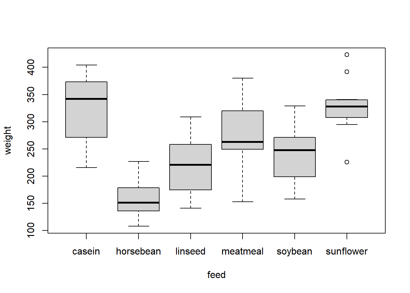
plot(weight ~ feed_soybean, data = chickwts) 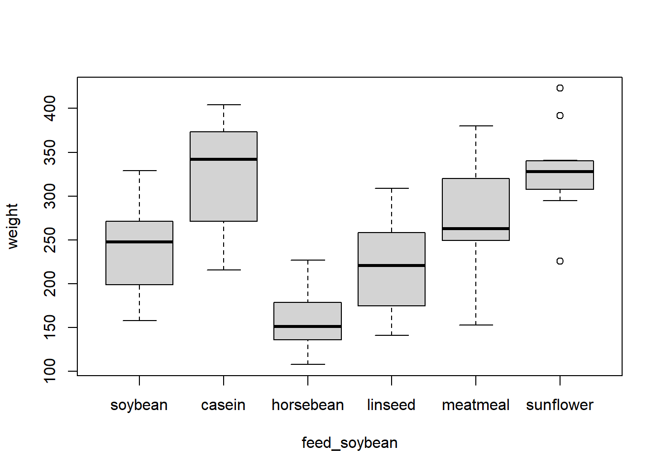
plot(weight ~ feed_reordered, data = chickwts) 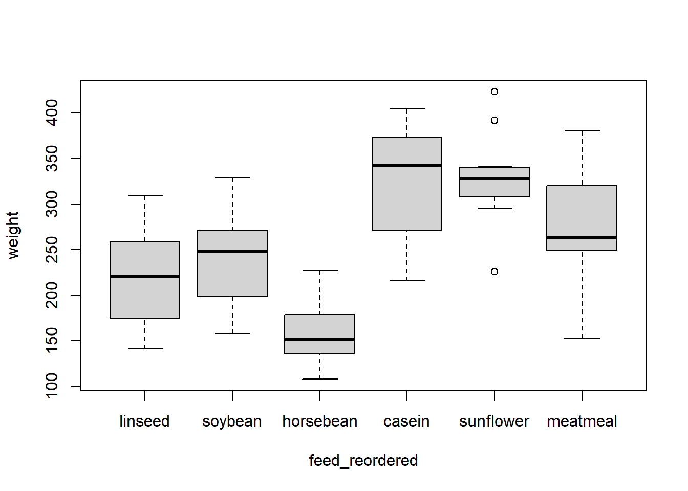
When we fit linear models and take a look at the coefficients, we will notice that the intercept changes (since it is the predicted value of the reference category) as do the coefficients for the other levels of feed (since each one is an offset to the reference category's predicted value in that model).
coef(lm(weight ~ feed, data = chickwts)) (Intercept) feedhorsebean feedlinseed feedmeatmeal feedsoybean feedsunflower 323.583333 -163.383333 -104.833333 -46.674242 -77.154762 5.333333 coef(lm(weight ~ feed_soybean, data = chickwts)) (Intercept) feed_soybeancasein feed_soybeanhorsebean feed_soybeanlinseed feed_soybeanmeatmeal 246.42857 77.15476 -86.22857 -27.67857 30.48052 feed_soybeansunflower 82.48810 coef(lm(weight ~ feed_reordered, data = chickwts)) (Intercept) feed_reorderedsoybean feed_reorderedhorsebean feed_reorderedcasein feed_reorderedsunflower 218.75000 27.67857 -58.55000 104.83333 110.16667 feed_reorderedmeatmeal 58.15909 Recoding
Recoding, or relabeling, is changing the labels on our factors. To do this, we can supply fct_recode() with our factor and a series of new_label = current_label pairs. Anything we do not name will be left in its existing state.
For example, we could make another factor in chickwts where we change "sunflower" to "experimental_feed":
chickwts$feed_recode <- fct_recode(chickwts$feed, "experimental_feed" = "sunflower") To confirm that it worked, make a table of the original and new variables:
table(chickwts$feed, chickwts$feed_recode) casein horsebean linseed meatmeal soybean experimental_feed casein 12 0 0 0 0 0 horsebean 0 10 0 0 0 0 linseed 0 0 12 0 0 0 meatmeal 0 0 0 11 0 0 soybean 0 0 0 0 14 0 sunflower 0 0 0 0 0 12 We can see that "sunflower" from chickwts$feed corresponds to "experimental_feed" from chickwts$feed_recode.
Another situation where we might want to do this is if the current labels are uninformative, such as if education were coded as 1 through 4, and a codebook provided keys:
education <- factor(sample(1:4, 10, replace = T)) education [1] 2 4 3 4 1 3 4 3 1 4 Levels: 1 2 3 4 education <- fct_recode(education, "Less than High School" = "1", "High School" = "2", "Some College" = "3", "College Graduate" = "4") education [1] High School College Graduate Some College College Graduate Less than High School [6] Some College College Graduate Some College Less than High School College Graduate Levels: Less than High School High School Some College College Graduate If we want to make systematic changes to our factor, we can use the fct_relabel() function. The first argument is still our factor, but the second argument should follow the pattern ~ function(.x), where .x is shorthand for our factor. To make all of chickwts$feed uppercase, we can use toupper():
fct_relabel(chickwts$feed, ~ toupper(.x)) [1] HORSEBEAN HORSEBEAN HORSEBEAN HORSEBEAN HORSEBEAN HORSEBEAN HORSEBEAN HORSEBEAN HORSEBEAN HORSEBEAN LINSEED LINSEED [13] LINSEED LINSEED LINSEED LINSEED LINSEED LINSEED LINSEED LINSEED LINSEED LINSEED SOYBEAN SOYBEAN [25] SOYBEAN SOYBEAN SOYBEAN SOYBEAN SOYBEAN SOYBEAN SOYBEAN SOYBEAN SOYBEAN SOYBEAN SOYBEAN SOYBEAN [37] SUNFLOWER SUNFLOWER SUNFLOWER SUNFLOWER SUNFLOWER SUNFLOWER SUNFLOWER SUNFLOWER SUNFLOWER SUNFLOWER SUNFLOWER SUNFLOWER [49] MEATMEAL MEATMEAL MEATMEAL MEATMEAL MEATMEAL MEATMEAL MEATMEAL MEATMEAL MEATMEAL MEATMEAL MEATMEAL CASEIN [61] CASEIN CASEIN CASEIN CASEIN CASEIN CASEIN CASEIN CASEIN CASEIN CASEIN CASEIN Levels: CASEIN HORSEBEAN LINSEED MEATMEAL SOYBEAN SUNFLOWER As seen with toupper(), we can manipulate factor labels with any function we might use with a character vector, such as paste0():
questions <- factor(1:5) questions [1] 1 2 3 4 5 Levels: 1 2 3 4 5 questions <- fct_relabel(questions, ~ paste0("q", .x)) questions [1] q1 q2 q3 q4 q5 Levels: q1 q2 q3 q4 q5 Collapsing and Dropping
Another factor manipulation is reducing the number of categories, called collapsing. We can do this with fct_collapse(), and our collapsing follows the pattern new_category = c(current_category1, current_category2, ...).
For an example, let's make a factor from the letters vector, which contains 26 lowercase letters, and make a level called "vowels":
let <- factor(letters) levels(let) [1] "a" "b" "c" "d" "e" "f" "g" "h" "i" "j" "k" "l" "m" "n" "o" "p" "q" "r" "s" "t" "u" "v" "w" "x" "y" "z" let <- fct_collapse(let, vowels = c("a", "e", "i", "o", "u")) levels(let) [1] "vowels" "b" "c" "d" "f" "g" "h" "j" "k" "l" "m" "n" "p" "q" [15] "r" "s" "t" "v" "w" "x" "y" "z" We can see that we have fewer levels in let, since our vowels were collapsed into a single vowels level. The other levels were left as is. What if we wanted to combine all of these into a factor called "consonants"? We could try typing it all out: consonants = c("b", "c", "d", ...) but this could take a while.
A faster option is to get a vector of all levels except for "vowels" and then use this in fct_collapse(). We can get all elements of levels(let) except for the first one with [-1].
cons <- levels(let)[-1] cons [1] "b" "c" "d" "f" "g" "h" "j" "k" "l" "m" "n" "p" "q" "r" "s" "t" "v" "w" "x" "y" "z" let <- fct_collapse(let, consonants = cons) levels(let) [1] "vowels" "consonants" Another option we could have used from the beginning relies an additional argument in fct_collapse(), the other_level argument. Any unnamed levels will be assigned this level. Be sure that everything else should be together in a category first, though!
let <- factor(letters) levels(let) [1] "a" "b" "c" "d" "e" "f" "g" "h" "i" "j" "k" "l" "m" "n" "o" "p" "q" "r" "s" "t" "u" "v" "w" "x" "y" "z" let <- fct_collapse(let, vowels = c("a", "e", "i", "o", "u"), other_level = "consonant") levels(let) [1] "vowels" "consonant" At other times, we might have extra, unused levels in a factor, which can happen when we subset data. In this example, x still has "d" and "e" as levels even after these levels do not have any observations:
x <- factor(letters[1:5]) x [1] a b c d e Levels: a b c d e x <- x[1:3] x [1] a b c Levels: a b c d e The reason we want to drop these unused levels is that they appear in plots:
plot(x) 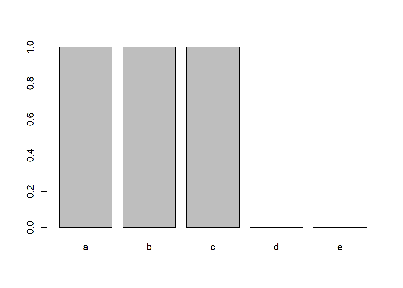
To remove them, simply use factor() to "reset" the factor and drop unused levels:
x <- factor(x) x [1] a b c Levels: a b c Now, we can plot x again to see that those levels have indeed been removed:
plot(x) 
Exercises
-
Releveling: Using the
irisdataset, plot counts by factor level withplot(iris$Species). Now, relevelSpeciesso thatversicoloris the reference (first) category. Plot it again. What do you notice? -
Recoding: In the
mtcarsdata, all the variables are numeric. Convertvsto a factor, where 0 has the label "V-shaped" and 1 has the label "Straight". -
Collapsing:
mtcars$cylhas three different values: 4, 6, and 8. Convert it into a two-level factor, where 4 and 6 share the label "Few" and 8 has the label "Many".
Advanced Exercises
- Use
row.names()to extract the row names ofmtcars. Create a factor from the first word in each element (the "make" of the car). (To separate a string, seestr_split()from thestringrpackage.) Create a table of make counts. Which is most common?
Source: https://sscc.wisc.edu/sscc/pubs/dwr/categorical.html
0 Response to "Differentiate Categorical Variables From Continuous Variables in Sas"
Post a Comment